
I've been working away at the Sea Mammal Research Research Unit(SMRU) for a year or so now. My main project has been to see if we can spot sea mammals using sonar. It's taken a while but I've finally managed to get somewhere and I'd like to share it with folks, in the hope it might help some of you out there, working on similar things.
Update. I gave a talk at EMF Camp 2024 on this topic. You can see the video here
I mean, it's a good question. Many sea mammals such as whales and dolphins make a fair bit of noise, so with hydrophones and clever maths we can figure out where they are. This is useful information when thinking about marine mammal protection and the effects human activity might have.
Thing is, seals don't make a lot of noise. It's also dark down there in the depths, so we need another method to spot them. Sonars are getting pretty good these days (at least to my layman's eye). The team had already put two of them down under the sea, watching a turbine in Scotland. They'd collected an awful lot of data and so I set to work.
The sonars we are using are the Tritech Gemini.
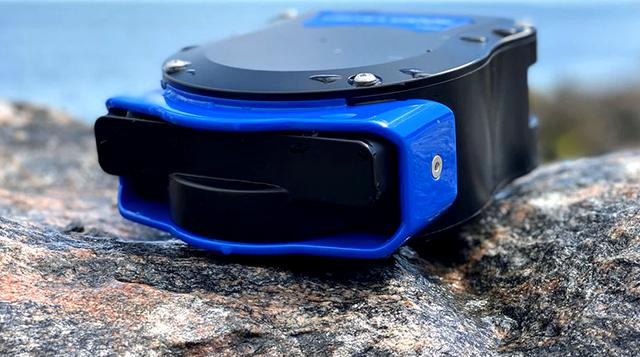
These things have 512 beams that shoot out a considerable distance (ours are set to around 55m). The framerate is about 8fps, or 4fps if two are interleaved on the same channel. The images are 512x1600 pixels - the height is dependent on the range setting. Each pixel is an intensity value stored as an 8bit unsigned int.
Typically, we like to view these things in a polar plot. This means distorting the rectangle into the 'fan-like' image.
The fan distortion algorithm can be sped up somewhat using something like Vulkan to write a GPU program that maps the rectangle onto a triangle strip, shaped like the fan. This works really well. However, the raw rectangles are much more amenable to analysis.
So this is the starting data. What's next is annotation.
This is the part of the gig that often goes un-celebrated - where do our lovely annotations come from? If we think about all the image classifiers out there, someone had to label all these images with terms like "a picture of a cat" or "a comic drawing of a dog". Our data are no different. SMRU uses a program called PAMGuard for many things. An initial detector was built that looks for related changes in sonar intensity. These detections are grouped into tracks. These tracks can be selected by a trained user and labelled as 'seal', 'fish' or any number of classes with a confidence score.
This process takes quite a long time and requires quite specific training and experience. In addition, the detector produces a lot of tracks that aren't of interest. Noise in the image, sediment off the seabed, debris, bubbles etc etc. In the end, around 1% of the tracks detected were annotated. So that's the initial bar we need to beat!
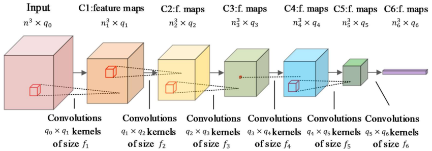
The first thing we can try and do is to try and classify these existing tracks, keeping just the ones that are useful. One such method is to use a convolutional neural network as shown in the figure below. The only difference is that rather than working with a 2D image, we are working on a spacetime volume; the third dimension being time.
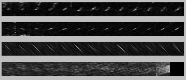
What we can do is look at the track and cut out a square image at that point. We then advance time by one frame and cut out another image. We stack these squares together to form a cuboid. We can visualise these images as a strip, such as in the image below:
With our data in place and our classifier written, we ran several experiments. Unfortunately, none of the models converged! It was quite disappointing but no matter how I stirred the statistical pot, the models just wouldn't work.
Chatting to my colleagues who performed the annotation, I figured that movement was quite important to classification. I wondered if spotting moving objects was a better approach? If we define a moving object as anything labelled as a seal or fish in our dataset, it should be possible to build a network that can pick them up.
There are quite a few methods for detecting moving objects. A lot of them involve removing the static background. One can use a number of methods found in OpenCV. The trouble with these approaches is they a) tend to work only with nice, static backgrounds such as roads or other man-made structures, b) they need some sort of variable to be set and that tends to be a hard cut-off and c) the objects are not identified as separate objects. There tends to be a lot of greeble or noise left over with these approaches, particularly in our dataset.
One A.I. method we can use to try and solve this problem is the U-Net. My hand-drawn diagram below shows the major components. The idea convolve over the image as before, then shrink the image down, convolve and repeat, until we get to the last layer where we - hopefully - have the most important information. The second step involves scaling the image back up again, hopefully with the segmentation we want. Much of this research comes from the medical imaging world. Things like X-rays, fMRI and such produce images where a particular area is of interest. A trained U-Net can take such an image and produce a mask of the same size with the important stuff inside the mask and everything else masked out.
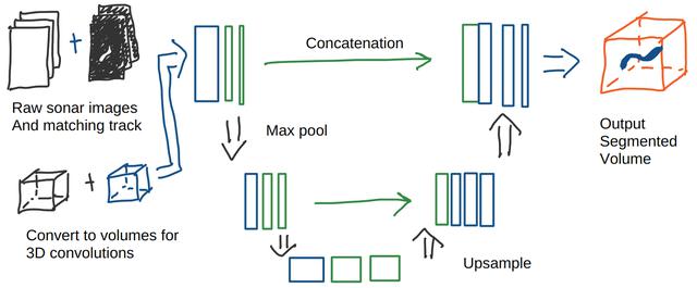
Now, again, imagine that instead of a single 2D image, we are working with our space-time volume. A moving object should create a diagonal 3D line through the volume. Indeed, any sort of line, except one parallel with the Z (time) axis. A 3D convolutional network should be able to pickup that pattern.
During a spare few hours, I put together a quick example. I generated some fake data, complete with fake ground truth and gave it a go. I was really surprised at how well it worked! I was amazed that it managed to still track the object when it was partially occluded.
I named the new network OceanMotion (of course!) and immediately set to with our data. Immediately I noticed something quite odd. I'd end up with loss curves like the one below:
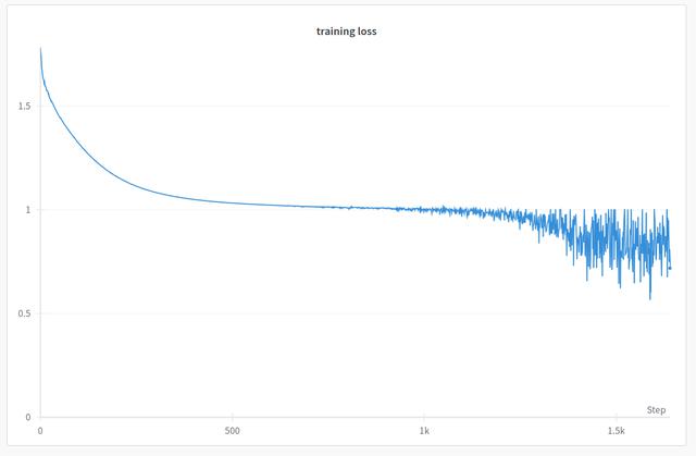
Typically, in deep learning A.I experiments, you get a nice, smooth(ish) curve that descends quite quickly initially, then tapers off around midway through and very gradually improves. The graph above shows that sort of curve initially, but then appears to fall apart. For a long while I was wondering what this meant?
Turns out the answer is due to the choice of loss function, or should I say, loss functions. The binary_cross_entropy_with_logits (BCE) function of Pytorch takes charge early on, reducing every pixel in the output to zero. This makes sense as our moving objects are really small compared to the background. Only a few pixels are classed as such. Therefore, the quickest way to get a good score is just to reduce everything to zero. This is what we see in the first part of the graph.
However, we use not one, but two loss functions. The Dice Loss (or more properly, the Dice-Sørensen coefficient) is very popular in segmentation tasks. It's common to use both the BCE loss and Dice loss together as this tends to give better results across the board. What we are seeing in that graph is the dice loss taking over. I still have no idea what makes this happen at this time, or why it tends to go up and down so much. Nevertheless, this graph shape became increasingly important as it tended to signal a good result.
Well indeed! How well did we do? Well, if we take the sonar video at the beginning of the article, you might be able to spot a moving object around the centre bottom of the video - scroll to 22:22 in the video above and you'll see what I mwan.
But here is the rub. Remember, we have lots and lots of data and only a small amount of it has something of interest in it. We need to run our model over a very long period and see how many false positives we end up with. We can reproduce all the nice tracks that agree with the human annotation, but there's no point if we end up producing a detection every 5 seconds.
Lets look at the longer term then. I designed a few experiments where I'd run the detector over 24 hours of data - sometimes a month of data. This could take a while to run - the current setup processes roughly 2 seconds of data per second (eventually, I'll speed this up). Nevertheless, such an experiment can run overnight. For every frame, I join up all the connected pixels into blobs and compute the bounding box. Saving just the bounding boxes keeps the amount of data down whilst retaining the most important features. We can then plot the number of pixels detected per frame on a big graph and see how we did.
The video at the top of the post shows me scrolling through the graph. Areas in red were ones with a sea mammal annotation. Areas in green had some other annotation (most likely fish). In this particular experiment, no red areas were missed, but there still seem to be a lot of false positives. Never-the-less, this model is performing very well. Only 1500 or so detections - that's about 1 per minute. This is a factor of 100 or more better than the original detector.
Quite often, a neural network might appear to be doing well, but it perhaps hasn't learned what you think it's learned. It doesn't take too much of a search to find example of where A.I has spectacularly failed.
I wondered if our neural network had just remembered the background. If so, such a model would not be much use if the sonar were placed elsewhere. Of course, at this point, it seemed only right and proper to introduce our old (one) friend, Cthulhu!
Yep! And not just a bit of fun either. If we change the background to something heretofore unseen (and possible sanity loss inducing!) and the network still gives a good result, then we know it's not sensitive to background (somewhat). The video below shows exactly this:
It's a pretty good result! Cthulhu is quite bright and so occludes the movement at first, but once the object leaves cthulhu's shadow, it is tracked correctly. Not bad at all!
There's still quite a lot of work to be done. Spotting a moving object is one thing and while it's likely to be a seal or fish (as that's what we are training on), our network doesn't tell us what this moving object is, and with what confidence. That's something we really should have. In addition, there are still too many small flashes of pixels that light up when there isn't any consistent movement there. These could probably be easily removed with some simple algorithms, or perhaps a little tweaking of the loss functions.
One approach I'm looking into is to combine a classifier on the high resolution images, with the current movement detector in a single network. Hopefully, the movement detector will push the classifier towards the regions with the information in, rather than the entire image. It's still a work in progress at the moment, but fingers crossed we can get a good result.
Folks at the SMRU Water Group have worked pretty hard on this. A lot of work was put into making the annotations in the first place; many hours clicking on tracks and deciding which tracks are worth considering. Something worth remembering when ever anyone does any A.I. or Big-Data work - where does the data come from and who put it together.