
Sequences appear a lot in biology, as you might expect. A and C and T and G, or ASP, GLY, VAL, PRO and many others. Looking for patterns in this data is half of the battle. Looking for patterns in the mountain of data is a herculian task. No wonder we are trying to teach machines to look for patterns. In my work, I'm trying to look for patterns in sequences of amino acids. It's not clear whether or not the sequences themselves have any patterns on their own, but it's worth a look.
Long-term short-term memory units, or LSTMs, are the new hotness in machine learning. Well, sort-of. They've been around for a while, but have recently found success in machine translation. Their power is in their memory. Each cell holds a small amount of state. It can chose to alter that state based on new information, or forget things it has previously learned. More importantly perhaps, any gradients being passed along tend not to explode or vanish over time.
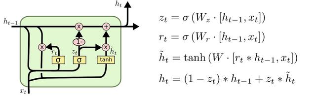
LSTMs come in a few flavours: the basic cell, cells with peepholes, Gated Recurrent Units (GRUs) and others. Tensorflow has support for most of these out of the gate.
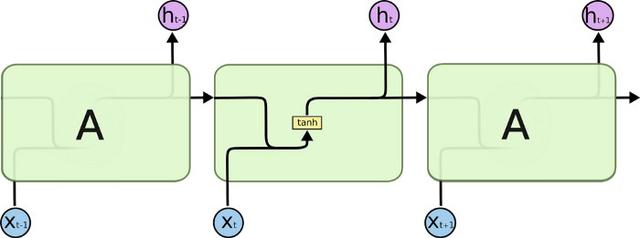
LSTM cells are combined into a Recurrent Neural Network; the output of one feeds the input of another. We decide how many steps we need, and unroll the network accordingly. We can do this dynamically based on the input sequences. At each step we can read the output or wait until we get to the end and read off the final result.
LSTM networks can also have multiple layers. The output from a particular step can feed into the corresponding step of the layer above.
LSTMs have often been used to translate human languages. In this case, you don't know how long the sentence is going to be before you need to start translating. In our problem space, however, we already know the sequence in it's entirety before we start. This means we can go from front-to-back and back-to-front.
This makes biological sense in some ways. When reconstructing loops, it's typical to start from both ends and meet in the middle, or compare the two results, built from either end. It's thought there may be some long range dependencies and we want to capture these if we can. An LSTM that goes in both directions provides a little extra coverage.
In some cases, we want to take a sequence of variable length, and output a single class or result. This is known as sequence classification. In such a case, we need to find the last relevant step, and use that to feed into our final layer. When we have considered all the steps, back and forward, we can return a result.
Another option is to return a result, or label, at each step. Every step is connected to the same set of weights and biases in our fully connected layer. This is where bi-directional networks really help us. The first step has no history to go on and may not be as accurate as successive steps. However, if we combine both directions, we should be able to mitigate that.
The advantage of labelling is a slightly more balanced network with fewer parameters, at least the networks I've tried. However, we can look at both and see which performs best.
Another method has become quite popular - sequence-to-sequence learning, or seq-2-seq. This is somewhat different to both approaches but has similar elements. I won't cover that in this post, but it's something I'll do in the future.
We first build a graph that takes a set of inputs of a certain kind. In our case, a bitfield that has the following dimensions:
[batch_size, max_length, 20]
We can more or less ignore batch_size for now. It's there because mini-batch gradient descent is now the sort-of standard as it were. 20 refers to the amino acid bitmask we are using, and max_length is the longest loop we are considering. It hovers around the 28 mark.
To construct an LSTM we build a set of cells, both in the forward and backward direction. We give each cell a certain size. This is the internal memory if you will. We then place each cell into a multi_rnn_cell container, one for each direction. We have a lot of choices of cells. Lots of people prefer the GRU cell as it has fewer parameters and is therefore faster to compute. I've left in the commented lines so you can see the options we have. The last line of the lstm_cell is a wrapper that adds dropout to the cell, which helps with overfitting.
def lstm_cell(size, kprob, name):
  ''' Return an LSTM Cell or other RNN type cell. We
  have a few choices. We can even throw in a bit of
  dropout if we want.'''

  #cell = tf.nn.rnn_cell.BasicLSTMCell(size, name = name)
  #cell = tf.nn.rnn_cell.LSTMCell(size, use_peepholes = True, name = name, activation=tf.nn.elu)
  #wrapper = tf.contrib.rnn.LSTMBlockWrapper
  #cell = tf.nn.rnn_cell.GRUCell(size, name=name)
  #cell = tf.nn.rnn_cell.BasicRNNCell(size)
  cell = tf.nn.rnn_cell.DropoutWrapper(cell=cell, input_keep_prob=kprob, output_keep_prob=kprob)
  return cell

graph = tf.Graph()
  with tf.device(FLAGS.device):
    with graph.as_default():
      x = tf.placeholder(tf.float32, [None, max_length, num_acids],name="train_input")
      num_classes = 36 * 36
      keep_prob = tf.placeholder(tf.float32, name="keepprob")

      # 3 layers of LSTM, each one half the size of the last
      sizes = [lstm_size,int(math.floor(lstm_size/2)),int(math.floor(lstm_size/4))]

      single_rnn_cell_fw = tf.contrib.rnn.MultiRNNCell( [lstm_cell(sizes[i], keep_prob, "cell_fw" + str(i)) for i in range(len(sizes))])
      single_rnn_cell_bw = tf.contrib.rnn.MultiRNNCell( [lstm_cell(sizes[i], keep_prob, "cell_bw" + str(i)) for i in range(len(sizes))])
Next, we initialise the state of the nets. I'm going with a default here.
initial_state = single_rnn_cell_fw.zero_state(FLAGS.batch_size, dtype=tf.float32)
initial_state = single_rnn_cell_bw.zero_state(FLAGS.batch_size, dtype=tf.float32)
One of the trickiest parts of such networks is we can't use the maximum length in any of our calculations. When we are working out the accuracy of the net, or the cost function, we need to know which values are actually real and which are just padding. Say we have a maximum length of 28, but the loop we are feeding in is 12 residues long. That means we need to pad out 16 positions with zeroes and make sure we don't consider them in our calculation. Not only that, but we need to figure out the lengths of each loop in the batch in order to pass this to the tensorflow dynamic rnn function. This is made complicated by the fact that we have to use tensorflow graph operations, or functions, in order to stitch it all together in a tight graph that can be differentiated and bundled onto our GPU. Fortunately, a nice chap on this website goes into quite the detail of how this can be done. I've reproduced the code here.
def create_length(batch):
  ''' return the actual lengths of our CDR here. Taken from
  https://danijar.com/variable-sequence-lengths-in-tensorflow/ '''
  used = tf.sign(tf.reduce_max(tf.abs(batch), 2))
  length = tf.reduce_sum(used, 1)
  length = tf.cast(length, tf.int32, name="length")
  return length
The following code finalises the LSTM part of the code.
outputs, states = tf.nn.bidirectional_dynamic_rnn(cell_fw=single_rnn_cell_fw,cell_bw=single_rnn_cell_bw, inputs=x, dtype=tf.float32, sequence_length = length)
# If we want a single direction LSTM we can use this line
#output, _ = tf.nn.dynamic_rnn(single_rnn_cell_fw, inputs=x, dtype=tf.float32, sequence_length = length)

output_fw, output_bw = outputs
states_fw, states_bw = states

# We concat the two passes here, but we could also add as well
output = tf.concat((output_fw, output_bw), axis=2, name='bidirectional_concat_outputs')
output = tf.nn.dropout(output, keep_prob)
If we decide to go with sequence classification, we need to find the last relevant output. Again, the same website above has a last relevant step function. This function works for multi-layer nets which is good, but it suffers a bit from the tf.gather line that can slow things down a lot. If one is using a GRU cell, or if you have a single layer, there is a much easier option of simply reading the last state. I've presented both here.
def last_relevant(output, length, name="last"):
  ''' Taken from https://danijar.com/variable-sequence-lengths-in-tensorflow/
  Essentially, we want the last output after the total CDR has been computed.'''
  batch_size = tf.shape(output)[0]
  max_length = tf.shape(output)[1]
  out_size = int(output.get_shape()[2])
  index = tf.range(0, batch_size) * max_length + (length - 1)
  flat = tf.reshape(output, [-1, out_size])
  relevant = tf.gather(flat, index, name=name)
  return relevant
The final layer also depends on what which approach we decide to use. For brevity, I've just included the process for sequence labelling. Here, we are looking for a set of probabilities at each step. These probalities correspond to the likelihood that this step has a certain label. In our case, we have 1296 classes, so our vector is 1296 long. Most of these values will be zero (we hope!) but a few will have higher scores, and hopefully, one will rise above the others. This final tensor has the following shape:
[batch_size, max_length, 1296]
It's worth noting here that we have two outputs - the raw logits and the prediction that has gone through a softmax function. The reason for this is we can't use the basic, in-built functions with our varying length inputs. I output both because there is one function that can do this, but I've not had a lot of success with it so far.
dim = sizes[-1] * 2

W_f = weight_variable([dim, num_classes], "weight_output")
b_f = bias_variable([num_classes], "bias_output")

# Flatten to apply same weights to all time steps.
output = tf.reshape(output, [-1, dim])
logits = tf.add(tf.matmul(output, W_f), b_f, name="logits")

prediction = tf.reshape(tf.nn.softmax(logits), [-1, max_length, num_classes], name="prediction")
output = tf.reshape(logits, [-1, max_length, num_classes], name="output")

test = tf.placeholder(tf.float32, [None, max_length, num_classes], name="train_test")
labels = tf.placeholder(tf.int32, [None, max_length], name="labels")
With our graph built, we can start training. This step is a little more complex however. We need to create a cost function that can mask out the padding results to create an accurate cost function. We can build such a mask from our input data. Essentially, we reduce the last dimension by summing it up, then calling the tf.sign function. Our cost function looks a little like this:
def cost_cat(gpred, gtest, glength, FLAGS):
  ''' Our error function which we will try to minimise'''
  mask = tf.sign(tf.reduce_max(tf.abs(gtest),2))

  cross_entropy = gtest * tf.log(gpred)
  cross_entropy = -tf.reduce_sum(cross_entropy, 2)
  cross_entropy *= mask

  cross_entropy = tf.reduce_sum(cross_entropy, 1)
  cross_entropy /= tf.cast(glength, tf.float32)
  cross_entropy = tf.reduce_mean(cross_entropy)

  return cross_entropy
We compute the cross entropy loss of the results. Most of this code from this website here, though I've adapted it to suit this particular problem.
There are various other details we can go into. Activation functions, different initialisation methods, regularisation techniques, layer sizes, etc. I've found that few of these things make too much differnce. Mostly it's the architecture and the data itself where the biggest gains are made. Much work still to go but so far, sequence labelling seems promising.